Theory and Principle of Advanced Ranging

By exploiting the unique properties of the LoRa® physical layer, the SX1280 LoRa modem can provide both long-range data communication and Round Trip Time-of-Flight (RTToF) distance measurements (Semtech Corporation). In this paper we present a new mode of distance measurement operation. This new mode is called Advanced Ranging.

Instead of actively exchanging timing information, Advanced Ranging allows us to passively overhear ranging exchanges. This feature allows gains in terms of both additional position information and, in the context of a sensor network, higher capacity.

To understand how Advanced Ranging works, and how these benefits can be realized, we begin by first re-examining conventional RTToF ranging.

Ranging

The basic principle of RTToF distance measurement is illustrated below. In this first diagram, a ranging request is sent from the ranging Master to the ranging Slave. At the same moment that the Master transmits its request, it also starts an internal timer.

The radio wave propagates at the speed of light and, if in range, will arrive and be received by the ranging Slave in the time it takes the wave to propagate from Master to Slave, T_MS.

The image on the left shows the communication between Master, M, and Slave, S. The image on the right depicts a snapshot of the moment the Master’s emitted ranging request arrives at the Slave. (We will follow these conventions throughout our explanation).

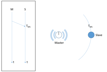
Figure 1: RTToF Principles: The Ranging Request

In a well-configured system, all of the processing delays are calibrated out [1] [2]. This means that we can consider the Slave acting as an active transponder that re-transmits a synchronised version of the ranging request. This ranging response takes time (T_SM) to propagate back from Slave to Master, which has timed the round trip delay to and from the Slave.

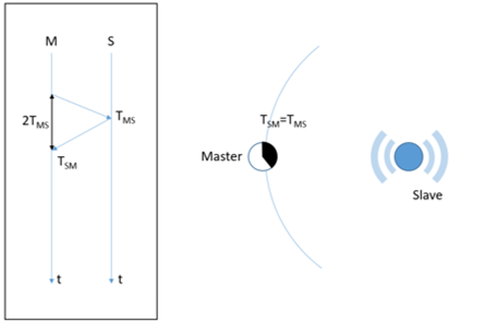
Figure 2: RTToF Principles: The Ranging Response

The propagation from Master to Slave, and back again, follows the same physical path, which means that the round trip delay represents twice the time taken to propagate from Master to Slave. Because we know that the radio wave has propagated at the speed of light, time and distance are equivalent. Therefore, the output of the ranging measurement is a distance, representing the radius at which we could expect to locate the Slave.

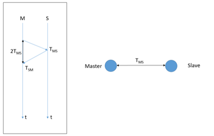
Figure 3: RTToF Distance Measurement

Ranging for Localization

The extension of RTToF ranging to localization is straightforward. In the image below, we indicate radios with fixed, known locations – known as anchors – with an anchor symbol. The mobile unit we are attempting to localize is in the center, which we will refer to as the tag.

Here, the anchors assume the role of ranging Master and perform a series of sequential ranging exchanges (as described above) to determine the distance from each Master to each Slave. We can then use these measurement results to trilaterate the location of the tag by finding the intersection of the range circles around each anchor, as illustrated:

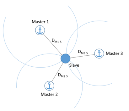
Figure 4: Distance Measurement Trilateration

Because the range is known at each Master, this example is well-suited to locating an object using a fixed infrastructure. However, it is worth noting that the roles of Master and Slave could be reversed between anchors and the tag. This second approach is better for circumstances where the mobile node is trying to determine its own location.

Ranging Performance

Localization, such as that depicted in the previous section, has a finite measurement accuracy. Recalling that accuracy is a measure of the absolute precision of the ranging operation, and that the precision is a measure of the spread of the results, the underlying precision of the round trip time-of-flight ranging of the SX1280 is shown below, in the Cramer-Rao Lower Bound (CRLB) model for theoretical Line-of-Sight (LoS) conditions [1]:

Figure 5: The Theoretical LoS Ranging Precision: the Cramer Rao Lower Bound (CRLB)

The diagram above portrays the theoretical ideal. However, the situation is complicated by the presence of multipath propagation. This is shown diagrammatically (in plan-view) below. In the following example, because the direct path between the Master and Slave locations is obstructed, the radio waves follow a reflected path. These reflected paths are all longer than the Line-of-Sight (LoS) path and so tend to result in an over-estimation of range. This effect is most marked when the path between Master and Slave is non-Line-of-Sight (nLoS). However, multipath effects can also be present in LoS environments, e.g., from walls and ceilings.

The following diagram shows how an nLoS environment between ranging Master and Slave results in multipath propagation.

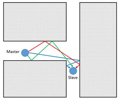
Figure 6: LoS Environment resulting in Multipath Propagation

Dilution of Precision

The position of the gateways relative to the object being located is critical in determining the resulting accuracy. The dilution of precision with respect to the location of an object is based upon the geometry of the anchor infrastructure. This is known as the geometric dilution of precision (GDOP).

In our simplified case, we concern ourselves only with the two-dimensional (2D) horizontal dilution of precision (HDOP). The method for calculating the HDOP is beyond the scope of this paper; we follow the method outlined in [3]. Here, we take a hypothetical localization case with four anchor units and position them at a range of 5km—one each to the North, South, East and West—and calculate the resulting dilution of precision.

The results are shown below in 2D plan view, with the intensity of the color map showing the increase in HDOP, which corresponds to a reduction in precision. Interpretation of the figure is straightforward: we multiply the underlying precision, or spread of results, of our ranging location estimate by the HDOP to determine the resulting location precision. Thus an HDOP >1 implies a degradation in precision.

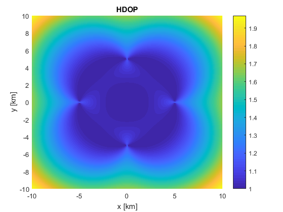
Figure 7: HDOP of Ranging Measurement

The implication of this theoretical result is that a tag will be a located with greater precision within the area delimited by the four anchors and, as we travel outside of this area, so the attainable location precision reduces.