documentation
The Immune System | Avoiding RF Interference with LoRa®
by Tim Cooper
Dealing with Uncertainty
Interference can be hard to predict, especially in a license-exempt ISM band, where the interferer could be another legitimate spectrum user or a service in a neighboring band. This is complicated further, as the severity of interference depends upon how much unwanted power couples to a receiver. This is as unpredictable as the environment where the radio is used.
This combination of hard-to-predict power levels and unforseen interference sources can lead to interference problems being discovered late in the design process – when they are the most expensive to correct. In this article, I tackle this problem and show you how to answer the deceptively simple question:
How likely is my radio to be immune to the interference it will encounter?
As the question implies, the answer will be probabilistic. Just as for estimations of range or packet error, knowing what level of error is tolerable is an important starting point. Other inputs are the likely sources of interference and the immunity performance of the radio. Ask yourself:
- Sources of Interference: What are the potential sources of interference in my application?
- Radio Receiver Interference Immunity: What kind of immunity can I expect from my radio?
There are two main ways of identifying potential sources of interference:
- Consulting the frequency allocations for the country or ITU region where the application is to be deployed [1]
- Surveying a typical application environment [2]
I will walk through an example based upon a LoRa® receiver, and predict the probability of how susceptible to interference the signals it receives might be. Contrary to how this is normally presented, my explanation should provide an intuitive indication of the level of risk.
Radio Receiver Interference Immunity
To understand which sources of interference may pose a problem, you need to have a basic understanding of receiver interference immunity. At the system level, there are three aspects to consider when examining interference:
- Interferer Frequency
- Interferer Power
- Interference Duty Cycle
Frequency and Power
To seek out interference we will look at the busiest, most heavily congested spectrum in the world and examine a LoRa modem operating in the global 2.4 GHz ISM band [3]. For this example, I will consider a LoRa radio in the presence of Bluetooth® Low Energy (BLE) interference. However, the broader principles presented here are applicable to any interferer in any band.
Figure 1 shows a typical low-IF receiver front end. Here we have a radio signal transduced by the antenna, then filtered by a low-pass filter before being amplified by the low noise amplifier (LNA). The amplified signal is down-converted to a low intermediate frequency (IF) before being band-pass filtered and sampled by an analog to digital converter (ADC). The ensuing channel filtering and demodulation is in the digital domain.
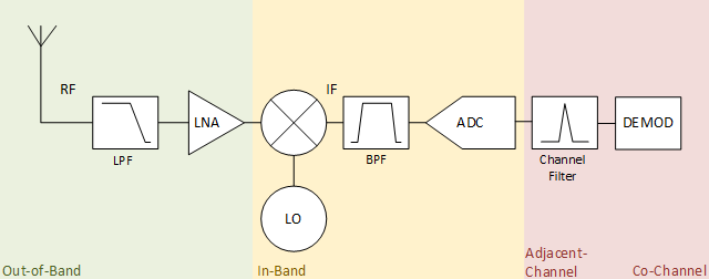
Figure 1. Receiver Block Schematic
Before we look at the rejection performance, let us examine the various filtering stages in our receiver because they are of vital interest when thinking about interference. Figure 2 shows the desired signal on the bottom, with the filtering on the same frequency scale just above it. The signal view is simple: we mix the desired signal from fRF down to our intermediate frequency fIF using a local oscillator (LO) at frequency fLO (Figure 2).
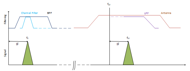
Figure 2. The frequency domain view of reception without an interferer
The filtering is all very standard, so I will not go into the detail of why each filter is there (for a good explanation see IF transceiver filtering [4]). However, it is important to note that the farther the interference is from the center frequency, the more cumulative rejection we receive from the increased filtering effort.
Because of this, interference is grouped into broad categories according to the frequency offset between the wanted and unwanted signal [5].
Absolute or Relative?
It is important to pay attention to the units used to quantify the level of interference immunity, namely, absolute or relative units. Figure 3 shows how interference immunity is usually measured.
The receiver under test connects to two signal sources, one wanted signal and the interferer. The sensitivity of the receiver is first measured in the absence of any interference, using only the wanted signal (for a specific bit or packet error rate). The power of the wanted signal will then be increased by 6 dB and the unwanted signal applied.
The power of the unwanted, interfering, signal is then increased until the same message error rate as for the senitivity test is obtained.
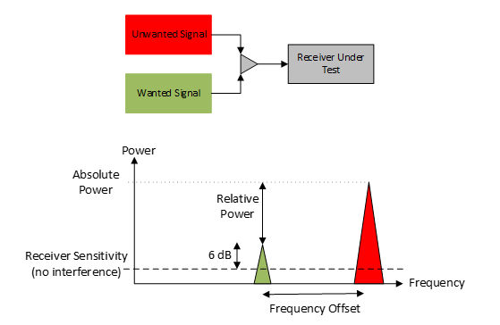
Figure 3: Quantification of Interference Immunity
The power of the interfering signal can either be recoded as an absolute power level or as the relative power of the interferer relative to the power of the wanted signal.
You can determine the frequency response of the interference immunity by varing the frequency offset between wanted and unwanted signal.
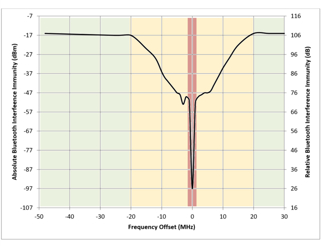
Figure 4. Interference Immunity of the LoRa Modem versus an always-on BLE interferer
To shed light on each of these interference categories, Figure 4 shows a plot of the real immunity of the LoRa modem to a Bluetooth interferer1.
Throughout this document, I will refer to the axis on the left hand side, which shows the absolute power of the BLE signal. The background colors in the plot correspond to the background colors in the receiver block schematic in Figure 1 and illustrate which elements are dominant in determining the immunity of the receiver at that frequency offset.
1. Full details can be found in Application Note: Bluetooth® Immunity of LoRa® at 2.4 GHz. [6] A very important consideration is that, unlike a real Bluetooth interferer, the unwanted interfering signal is always “on.” This is not representative of the “bursty,” packetized nature of a true BLE interferer.
Far from the Wanted Frequency: Out of Band Interference
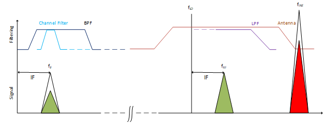
Figure 5. Receiver Blocking
How and why does a radio’s immunity change as a function of frequency?
Starting far from the wanted signal, over 20 MHz in our example, is the area highlighted in green in the plot of Figure 4 where the modem can still receive even in the presence of a -17 dBm BLE interferer. The element which limits the receiver performance in the presence of a high power signal are the LNA and input filter area highlighted in green in Figure 2.
Blocking is the phenomenon of a high-powered signal causing gain compression in the LNA. The unwanted signal saturates the LNA, reducing the LNA gain of both the high-powered blocking signal and the small-signal gain at the wanted frequency. The reduced amplification of the wanted signal (sometimes also combined with spectral regrowth in the baseband due to nonlinearity) reduces the receiver sensitivity.
The advantage we have for any interfering signal far out of band is that it will be attenuated by any front-end receiver filtering. Sources of filtering also include the oft-overlooked antenna, as well as the filtering of the low pass filter, which will further attenuate the signal.
Same Band: In-Band Interference
When the interferer is closer to the wanted signal (highlighted in yellow in Figure 4) we get between -17 dBm and -50 dBm of immunity. In this region, the rejection performance is a complicated mix of the blocking performance of the LNA, the frequency response of the mixer and the band-pass filter. As we get close to the wanted channel, the in-band rejection becomes limited by the RF phase noise of the local oscillator.
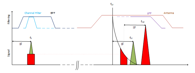
Figure 6. Reciprocal Mixing
Figure 6 shows the dominant contribution just within the channel filter stop band, a process known as reciprocal mixing. Here, the local oscillator (LO) phase noise folds into the wanted channel and limits the receiver sensitivity. An excellent description, not only of the process itself, but also the equations to derive an LO phase noise requirement can be found in Computing the LO Phase Noise Requirements in a GSM Receiver [7].
Image Rejection: At the Image Frequency Only
In the case of a Low-IF receiver, there is one last exception to handle: the image frequency. The down-conversion process mixes the wanted RF signal down to the intermediate frequency. In addition to this, the low-side (FLO – FIF) is down-converted to minus the IF. This complex signal folds into the channel filter, as can be seen in Figure 7.
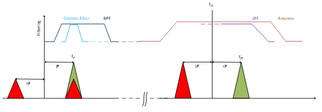
Figure 7. Image Rejection
The intermediate frequency of the SX1280 in receive mode is 1.625 MHz. This means that the image frequency can be found at twice the IF below the programmed RF center frequency, i.e. FRF minus 3.25 MHz. The image rejection can be seen in Figure 4, as a dip at 3.25 MHz below the RF center frequency.
Same Frequency: Co-Channel Interference
The worst case rejection (highlighted in red in Figure 4), with only -97 dBm unwanted signal power preventing reception, is with an interferer on the same channel. Referring back to our receiver block diagram, in this case all of the interference rejection comes from the demodulator, as the signal within the receiver channel filter (red) must discriminate between the wanted and interfering signal. The frequency domain view of this is shown in Figure 8:
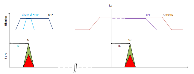
Figure 8. Co-Channel Rejection
While this is the worst case for interference because it has the lowest immunity, LoRa has the advantage of being able to receive signals below the noise floor and, equivalently, below interference (Figure 9).
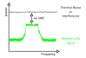
Figure 9. LoRa Reception is Possible with negative SNR
Unintentional Antennas
So far I have assumed that all of the sources of interference are arriving in the radio receive path via the antenna. It is important to note that there are other coupling mechanisms possible. A simplified example of which is illustrated below (Figure 10).
In the example below, we have two sources of iterference, a wireless router and a smart watch. These are generating interference on two different frequencies (shown in the leftmost plot) that arrive at the radio PCB with a certain field strength. Any metallic structure can act as an antenna – wanted or not! In this case, the unintentional antenna has a certain efficiency as a function of frequency (the middle plot).
The result is shown in the graph in Figure 11. The incident interference is transduced by the unintentional antenna formed by the PCB, and results in conducted interfering signals present on the board.
The remedy to this is adhering to good RF design principles and using board-level sheilding where appropriate [4].
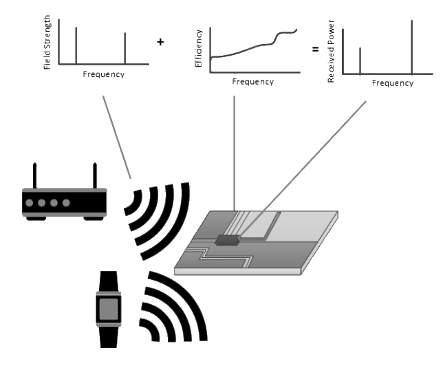
Figure 10. Interference can couple to the radio from paths other than the radio antenna
Distance not Power
While the interference immunity curve of Figure 4 is useful for comparing systems, it does not give a sound insight into how it can cope with interference. The plots can give more insight about the risk of interference when we convert these interference immunity figures into distances. This gives us information, both about what to really expect, and that we can use in our design process.
In converting to distance, my only assumptions are that the interferer is line-of-sight, and I estimate a conservative 20 dB of coupling loss between the LoRa antenna and the BLE antenna, even at zero distance. A quick check of this in a lab shows 25 dB of loss between a pair of Taoglas ceramic antennas at aproximately 1 cm of separation (Figure 11).
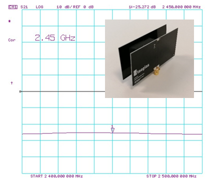
Figure 11. 25 dB of Measured Close Range Coupling between a pair of 2.4 GHz Taoglas chip antennas at 1 cm (Inset: measurement setup)
My final assumption is that the Bluetooth transmitter EIRP is 0 dBm.
Based upon these assumptions we can calculate the distance at which the absolute interferer power will be generated at the receiver input. I start by calculating an interferer link budget, L, in dB.
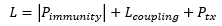
Where Lcoupling = 20 dB, Pimmunity is the absolute blocking immunity of Figure 3 and Ptx is 0 dBm.
Taking the resulting link budget, we plug it into a rearranged free-space path-loss equation to calculate the separation distance, d at which our receiver would be overpowered by the BLE interferer.
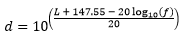
Where f is the frequency in Hz (2.45 GHz).
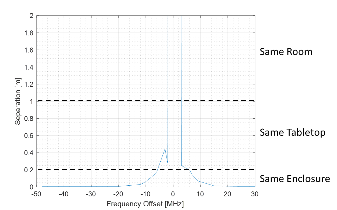
Figure 12. Interference immunity of an always-on interferer: translating the interference rejection into distances can help interpretation
The plot of d – the distance at which my BLE interferer blocks our LoRa communication – versus the frequency offset is shown in Figure 11. The probabaility of experiencing interference from our Bluetooth transmitter appears low at ranges, when there is more than 1 meter separation between the LoRa and BLE radios, with only six percent of the 80 MHz band where there is the possibility of interference. Only 15 percent of the band would be interfered with when the devices are from 20 cm to 1 m apart.
You should now have a more intuitive feel for when and how our receiver could be affected by interference. But this is still only part of the story. This plot in Figure 11 is for an always-on interferer. I have ignored the infleunce of when the interference is present.
Time on Air
To calculate the probability of collision (i.e. a LoRa packet coinciding with a BLE packet), we need to consider the time-on-air of each. Let us assume we will receive a packet with the following format, on a single channel (Figure 13).
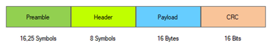
Figure 13. LoRa Packet Format of the Purpose of our interference immunity study
At SF12, 200 kHz bandwidth, this equates to a time on air of 892.8 ms and a LoRa symbol time of 20.2 ms.
We compare this with an example of BLE time on air from BLE v4.2: Creating Faster, More Secure, Power-Efficient Designs—Part 1 [8]. Here, I assume the worst-case data transfer possible in Bluetooth 4.2, i.e. a very high data transfer from an interfering radio that is very close to our LoRa radio.
Assuming a hopping pattern over all 37 non-advertising channels of the BLE channel plan, we can expect 2.12 ms of transmission time, repeating every 277.5 ms.
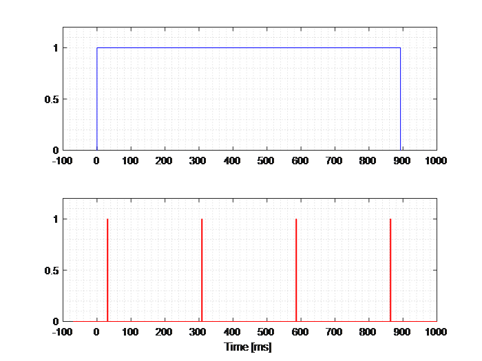
Figure 14. The Duty cycle of the BLE interferer (red) versus a single LoRa packet (top) on a single channel
In the general case, the product of the probability of collision is used to determine the immunity. In our case, a packet collision is guaranteed. Meaning that if we have a collision, and are within the range of power that will cause interference, we will lose our LoRa packet.
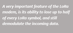
A very important feature of the LoRa modem, is its ability to lose up to half of every LoRa symbol, and still demodulate the incoming data.
Interferer Duty Cycle vs LoRa Symbol Time
In LoRa systems this is a frequent occurrence. LoRa allows us to trade-off time-on-air for increased sensitivity. This implies interference with much lower time-on-air (higher data rate than LoRa). A very important feature of the LoRa modem is its ability to lose up to half of every LoRa symbol and still demodulate the incoming data. Recalling that the symbol time is given by:

In our 2.4 GHz example, we can see that 2.12 ms BLE packet duration versus our 20.2 ms LoRa symbol period means we should still be able to recover a LoRa symbol that has been blocked by a BLE packet.
To demonstrate the immunity of the LoRa modem to “bursty” interference, I performed a LoRa co-channel rejection measurement. Contrary to previous measurements, this is done with a pulsed interferer. On the X-axis, instead of varying the frequency offset, I am varying the “on” time of the interferer. The timing diagram in Figure 15 illustrates this.
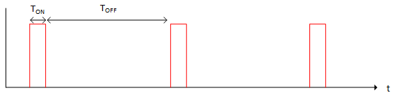
Figure 15. Pulsed Interference with a Fixed Duty Cycle
In this example, the interferer will always be on the same channel, and it will have a fixed duty cycle of 10 percent. Instead of changing the frequency variable, we are changing the “on” time TON (so consequently also the “off” time), and retaining our fixed duty cycle of 10 percent.
Duty cycle = TON / (TON + TOFF)
Although these specific measurements were performed with a pulsed CW interferer (no modulation) and in the sub-GHz band, the measurement results apply to any LoRa modem. The exact settings used were:
- LoRa SF12
- FEC Coding Rate = 4/5
- LoRa BW = 125 kHz
- LoRa Symbol time = 32 ms
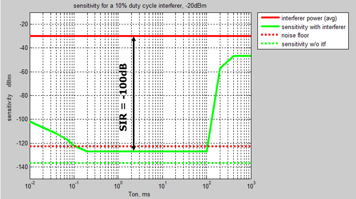
Figure 16. Measured Pulsed Interference Rejection of the LoRa Modem
Figure 16 shows the resulting measurements. The red line at the top of the graph shows the power level of the unwanted interfering signal. The solid green line shows the minimum LoRa signal level we can receive in the presence of our pulsed interferer.
The incredible result here is that, once our interference pulse duration is less than about 50 percent of the symbol time, we win a 100 dB relative signal-to-interference ratio (SIR). That is the ability to receive a signal a mere 10 billionths of the blocking power. With 100 dB of wanted signal-to-interference in response to bursty interference, the overall rejection of Bluetooth by our LoRa modem equates to a total immunity beyond 2 cm. (Figure 17. Note the change in Y-axis units.)
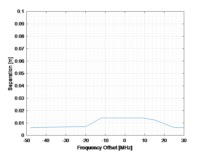
Figure 17. LoRa Modem Rejection of Frequency Hopped BLE Interfernce
Conclusion
The general method and principles outlined here are applicable to any radio technology. Using our example of LoRa in the 2.4 GHz band in the presence of BLE interference, we have seen a way of converting interference immunity data to an easier-to-interpret immunity-versus-distance plot.
We then looked at the worst-case scenario permitted in the BLE 4.2 specification, where the LoRa receiver is next to a BLE transmitting the highest volume of data possible. This additional timing information allowed us to derive the interference-immunity versus distance plot including the additional 100 dB of isolation due to the LoRa modem.
This finally allowed us to determine that our LoRa receiver at SF12 200 kHz would have to be within a couple of centimeters of the BLE transmitter to experience any kind of interference.
Semtech, the Semtech logo, LoRa, and LoRaWAN are registered trademarks or service marks of Semtech Corporation or its affiliates.
The Bluetooth® word mark and logos are registered trademarks owned by Bluetooth SIG, Inc.
References
[1] ITU Channel Plan: https://www.itu.int/en/ITU-R/terrestrial/fmd/Pages/frequency-plans.aspx
[2] Spectral survey examples:
https://www.keysight.com/upload/cmc_upload/All/Site_Survey_Webcast.pdf
[3] Congestion in the 2.4 GHz ISM band
https://blog.aerohive.com/suffering-from-wi-fi-congestion-dual-5ghz-radios-can-help/
[4] Transciver architectures and filtering can be found in Pozar, “Microwave and RF Design of Wireless Systems”, John wiley & Sons, 2001 ISBN 0-471-32282-2
[5] Categories of interference as defined by the CEPT:
https://ecocfl.cept.org/display/SH/1.2.11+In-band%2C+out-of-band%2C+spurious%2C+unwanted+emission
[6] Application Note: Bluetooth® Immunity of LoRa® at 2.4 GHz
(https://www.semtech.com/uploads/documents/AN1200.44_Bluetooth_Immunity_of_LoRa_at_2.4_GHz_V1.0.pdf)
[7] Emanuel Ngompe Conexant app note: Computing the LO Phase Noise Requirements in a GSM Receiver (https://archive.org/details/ComputingTheLOPhaseNoiseRequirementsInAGSMReceiver)
[8] BLE v4.2: Creating Faster, More Secure, Power-Efficient Designs—Part 1 (https://www.electronicdesign.com/communications/ble-v42-creating-faster-more-secure-power-efficient-designs-part-1)
[-] Receiver linearity and blocking IP2 and IP3 Nonlinearity Specifications for 3G/WCDMA Receivers https://highfrequencyelectronics.com/Jun09/HFE0609_Liu.pdf