documentation
Data Packet Transmissions
The previous sections have provided general information about payload size, and how and when to segment data into different packets. This section provides specific information about the update logic and payload contents to maximize the transfer of useful information using minimal transmission bandwidth. When you consider transmitting data, ask yourself these questions:
- How often should data be sent?
- What should the data format be?
- How many digits of precision is enough?
- What kind of payloads should not be sent?
The following sections will provide some suggested answers to these questions. While there is plenty of room for creativity and deep thinking, these guidelines are meant to help avoid mistakes in creating efficient payloads.
Minimum Update Rate of Information
A critical aspect of a data plan is making sure that you capture the necessary dynamics of the system you are trying to observe. Much research has been conducted regarding how to make a minimum number of samples in a system. The Nyquist-Shannon sampling theorem provides an optimal sampling of an analog signal to completely reconstruct the signal from its samples. Shannon’s version of the theorem is:
If a function x(t) contains no frequencies higher than B hertz, it is completely determined by giving its ordinates at a series of points spaced 1/(2B) seconds apart1.
Therefore any sampling rate higher than 2B is sufficient to capture the original signal. For highly periodic physical measurements, if the principle measurement is the height of the tide, which has an average period of 12.42 hours, a sampling rate of 6.21 hours will result in an accurate representation of high and low tides. If you have a model of how the measured quantity varies between updates (the tide level between the 6.21-hour sample in this case) you can form a contemporaneous estimate “right now” and any point between the samples. Without the model, you would need to sample more often to establish the current value of the measured quantity. When repeatability and a model of the measured quantity exist, there is a defined minimum sampling limit (2B). When there is no established periodicity and no model for the measured quantity, Nyquist-Shannon does not offer adequate insight.
Applications will impact how and when you make measurements. The physical system will influence the design of the application. If you are performing measurements in a system when you do not (or cannot) have a model of how a measured quantity will vary, the needs of the application will drive the sampling rates. For example, temperature readings in a room with manual controls. You may not know when heating or cooling occurs, so you will not know beforehand when there might be a significant change in the temperature. As a result, you need to sample at a rate that is adequate for your application. If you want to respond to an over/under-temperature event in less than five minutes, sample at least every five minutes. To address this issue, you can use just-in-time (JIT) and event-driven sampling. By employing event-driven sampling, the number of data transmissions can be dramatically reduced without loss of data variation. This approach can help you avoid transmitting a large amount of repeated data when there is a detailed history of events.
Just-in-Time Measurements
Many applications and sensors can use event-driven measurements or alerts. These sensor application examples include, but are not limited to:
- Door or window open/closed
- Leak detected
- Desk or room occupied/empty
- Low tank level warning
- Smoke or fire alarm
- Light/dark detection
- Button press
In each sensor application example, there is some event or state change that the sensor is trying to capture. The important information is about the change of state, not some value between updates. For example, when detecting if a window is open or closed, the important information is when the door or window goes from opened-to-closed or closed-to-open. We can assume that the time in-between events, the door or window was in the same state as the previous update. Note: It is important to monitor the sensor state; a depleted battery and can no longer send its state change information. For more information, see Heartbeat Messages.
However, there is another use of JIT updating; sending new data when an application significant change happens in any type of sensor. Even sensors that make continuous measurements, such as pressure, temperature, tank levels, etc. can be used by hitting critical fixed or relative levels. For example, if an application monitors pressure in a system and the most important factor is whether a critical pressure level is exceeded, sending the pressure level when that level is met will be a better solution than waiting until the next update is due. Extending this concept, a device could send data only when the limits are crossed, turning the continuous sensor into a discrete sensor such as the door open/close sensor. This is beneficial if the amount of power to make a measurement is significantly less than the power to transmit a measurement. In this way, a sensor can make many measurements and transmit data only when significant new information is available but allowing for continuous monitoring of a crucial environmental quantity. This approach of monitoring a quantity can also be used for delta-updating; if a value changes by some fixed value, you can transmit an update. For example, if you are monitoring temperature you could set a delta temperature (e.g., two degrees Celsius). When the temperature varies more than the delta setting since the last update, a new update is sent, and an updated reference temperature is set (see Figure 4).
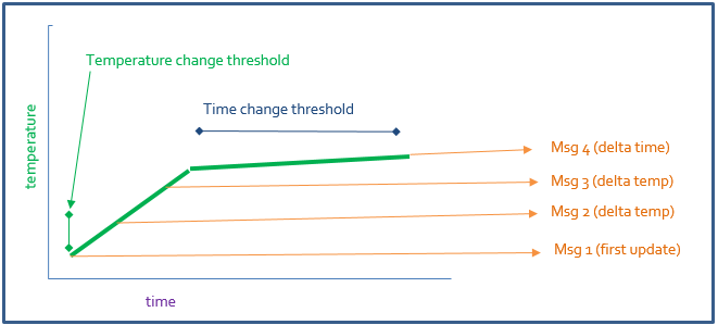
Figure 4: Delta updating
This suggests that, even when a measurement is a continuous-type of function, it can be updated as if it were a discrete, observation-based function, based on rules in the remote device. For example, temperature, pressure, fluid flow rate, and so on. These rules must be driven by the application and the capabilities of the device, but using JIT updating for just about any device can lead to dramatic transmit times which in turn leads to less time on-air for each device and potentially dramatic power consumption reduction. When you evaluate application requirements; review if there is a need to report a measurement every
Bit Packing
Bit packing is another critical aspect of maximizing data transfer in the smallest number of bits. Bit packing takes advantage of the binary data transmission of the payload (i.e., the bits of the payload are sent one at a time) to provide a compact stream of information. A key element in effective bit packing is making sure that you provide the appropriate scale and precision. For example, you may want to provide the current battery voltage of a device. The available precision may be 100 mV but the application requires 0.1V precision. You know that the battery will operate between 2.6V (below which the device shuts off) and 4.1V (when the battery is fully-charged). Between 2.6V and 4.1V there are 15 0.1V steps so you can represent the voltage by using the following calculation:
V = 2.6 + 0.1 * ν {ν: 0-15}
This means that a voltage with a precision 0.1V and a range 2.6V to 4.1V can be transmitted with only four bits (hex 0xF or 0-15). Compare this to the character array of “3.1” which comprises three individual characters, that are sent in three separate bytes: “3”, then “.” then “1”. This would be transmitted as ASCII-code values of 51,46,492. As you can see, transmitting three individual characters takes three bytes, or 24 bits (ASCII), versus four bits (Hex). The character-representation has the advantage of being able to represent 0.0V through 9.9V. The middle byte does not really need to be sent, it is always “.”=46 ASCII decimal. For more information, see Redundant Information and Text. The effective penalty is 12 bits. If the minimum necessary data can be sent in four bits; sending more bits than absolutely required for the same data is wasteful—both in air-time and in power consumption. You can modify the formula, the number of bits and the precision to meet various requirements for range and accuracy. Many physical measurements that seem like they can take lots of data bits can be compressed into smaller bit representations. In addition to these examples, Table 4 shows a variety of bit-packing examples for common physical and other measurements.
| Quantity | Desired Quantity | Bit Packing Formula | Bits required | Range | Precision |
| Time3 | Arbitrary date and time to second | T = seconds from Jan 1, 1970 00:00:00 | 32 | Jan 1, 1970 00:00:00 to Jan 19 2038 03:14:07 | 1 second |
| Temperature | Temperature wide range |
T =0.5*( t -80) |
8 | -40 C to +87.5 C | 0.5 C |
| Temperature | Temperature narrow range |
T = 0.25*(t-40) |
8 | -10 C to +53.75 C | 0.25C |
| Temperature | Temperature course |
T = 4*(t-1.25) |
4 | -5 C to +55 C | 4C |
| Voltage | Voltage wide range |
V = 0.1 * v |
8 | 0 to 25.5 V | 0.1V |
| Voltage | Voltage narrow range |
V = 0.1 * (v+26) |
4 | 2.6V to 4.1V | 0.1V |
| Battery level | Battery % precise |
P = 100% * p/15 |
4 | 0-100% | 6.67% |
| Battery level | Battery % course | P = 100% * p/3 {p:0-3} |
2 | 0-100% | 33.33% |
Table 4. Bit packing examples
Another typical value pair sent by sensors is latitude and longitude. These values are often represented in decimal degrees.
Note: Be sure to match the precision of the measurement with the precision of the data being transmitted. For example, if your position estimation device (GPS or GNSS) has a precision of one meter, providing any additional precision beyond one meter does not add additional value; it simply adds bits to the data packet. Additionally, if the accuracy of the system is limited in some way (from systematic errors in the estimation process), that will also limit the necessary precision that needs to be transmitted in the data packet. For standard GPS or GNSS applications, the best-case scenario for accuracy is about two meters. However, this will depend on the application and location determination technology. At the same time, taking into account the general accuracy and precision of a standard GPS or GNSS receiver, two meters is a good target for data precision in latitude and longitude transmissions4. Keeping this in mind, when looking at different scales for decimal degrees as shown in Table 5, five decimal places can achieve nearly one meter of precision in mid-latitudes (0.787m at 45N/S) and very nearly one meter at the equator (1.1132m). By going to six decimal places, the transmission precision can be a fraction of a meter. This fits easily in a 32-bit signed value. See the following example:
- Latitude, Longitude = (37.385909,-121.925453)
- Integer Latitude = (37.385909+90.0) * 1.0e6 = 127385909 (dec) = 0797C135 (hex)
- Integer Longitude = (-121.925453+180.0) * 1.0e6 = 58074547 (dec) = 037625B3 (hex)
Note: The latitude was mapped between 0 and 180 and longitude from 0-360. When converting back, the values need to be backed out:
- Integer Latitude = 127385909 (dec) = (127385909) / 1.0e6 = 127.385909-90.0= 37.385909
- Integer Longitude = 58074547 (dec) = (58074547) / 1.0e6 = 58.074547-180.0= -121.925453
|
Decimal places |
Decimal degrees |
DMS |
The object that can be clearly recognized at this scale |
N/S or E/W at the equator |
E/W at 23N/S |
E/W at 45N/S |
E/W at 67N/S |
|
0 |
1 |
1° 00′ 0″ |
Country or large region |
111.32 km |
102.47 km |
78.71 km |
43.496 km |
|
1 |
0.1 |
0° 06′ 0″ |
Large city or district |
11.132 km |
10.247 km |
7.871 km |
4.3496 km |
|
2 |
0.01 |
0° 00′ 36″ |
Town or village |
1.1132 km |
1.0247 km |
787.1 m |
434.96 m |
|
3 |
0.001 |
0° 00′ 3.6″ |
Neighborhood, street |
111.32 m |
102.47 m |
78.71 m |
43.496 m |
|
4 |
0.0001 |
0° 00′ 0.36″ |
Individual street, land parcel |
11.132 m |
10.247 m |
7.871 m |
4.3496 m |
|
5 |
0.00001 |
0° 00′ 0.036″ |
Individual trees, door entrance |
1.1132 m |
1.0247 m |
787.1 mm |
434.96 mm |
|
6 |
0.000001 |
0° 00′ 0.0036″ |
Individual humans |
111.32 mm |
102.47 mm |
78.71 mm |
43.496 mm |
|
7 |
0.0000001 |
0° 00′ 0.00036″ |
Practical limit of commercial surveying |
11.132 mm |
10.247 mm |
7.871 mm |
4.3496 mm |
|
8 |
0.00000001 |
0° 00′ 0.000036″ |
1.1132 mm |
1.0247 mm |
787.1 µm |
434.96 µm |
Table 5. Precision of Decimal Degrees5
Encoding
Encoding refers to taking the original representation of data and converting it to a different form. For example, the scheme called “Base64 encoding,” takes binary data and converts it to printable ASCII text for transmissions on systems that can only support text. Generally encoding is not needed–and may well be contraindicated–for systems that can support binary data transmissions, such as LoRaWAN. However, there is something similar that can help maximize data content: lookup tables. Certain data exchanges use lookup tables such as sending timescale information (e.g., 10 seconds, 1 minute, 3 hours, etc.). For example, if you want a user to be able to select update rates between 10 seconds and one day, you could use 10 seconds as the base quantity and index that from one to 8640 (the number of ten-second blocks in a day). The number 8640 takes 14 bits to transmit. However, if you only wanted to provide certain options like, 10 seconds, one minute, one hour and one day, you could relay information in two-bits (four binary states): (0 0)=10 seconds, (0 1)=one minute, (1 0)=one hour, and (1 1)=one day. This spans the same range with 12 fewer bits; the cost of not being able to represent an arbitrary number of 10-second blocks of time. Adding an additional bit provides eight states and another gives you 16. If only certain fixed values in a continuous range of interest need to be sent, an interface design can save many bits for effectively the same amount of information being transferred.
Redundant Information
An example of redundant information is sending identical temperature measurements every five seconds. Even if there is a requirement for dynamic data updates, there are better ways than filling the data stream with the same information repeatedly. For more information, see Just-in-Time Measurements. Another example of redundant information is the frequent repetition of configuration information. It is useful to send status information about the state of the device. However, sending a configuration byte every two minutes that states that the device will send an update every two minutes is pointless. A key aspect of maximizing data delivery with a minimum of data bits is knowing when to confirm settings and when to allow the user to assume the settings are the same as the last confirmation. If the settings can only be changed through over-the-air commands, send a confirmation of the settings when they change. After that, send confirmations no more than every 24 hours.
Text
The LoRa or LoRaWAN transmissions are sent as in binary data. Printable text is not very efficient for transmitting data. For example, view the printable ASCII text in Table 62, the “printable” characters go from 32 decimal to 126 or 94 values out of a 256 valued binary byte. This is a 36.7 percent use of the available values. If you limit the values to alphanumeric values plus the space character, the number of remaining characters drops to 63, reducing of the available values down to 24.6 percent. By limiting the data type to text, there is a potential loss of data efficiency ranging between 63.3 percent and 75.4 percent—before taking into account any other factors. Say we know that the first field in a given packet is voltage. If the field is formatted as: “Voltage=3.1V” then having both the “Voltage” string and “V” is redundant, since we already know this field is voltage from its position in the packet. Additionally, this string takes 12 bytes (96 bits) to transmit. We know from Bit Packing that a voltage with a precision of 0.1V between 2.6V and 4.1V can be sent in as few as four bits; or a half-byte—a 96 percent savings. Also, sending text in data fields usually results in highly redundant data with text phrases like “Voltage,” “V,” or “temperature” repeated in every packet. For more information, review the Redundant Information section. The only type of application packet that should be sent as text is a text-message application. As appropriate, compression should be used on that text6.
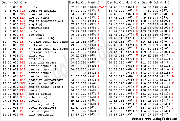
Table 6. ASCII table
Heartbeat Messages
Heartbeat messages allow for a regular but infrequent interval of messages that confirm a device can still report. There are many reasons why a device might no longer report to a LoRaWAN network. For example, the device may have been removed from the local network, the battery may be dead, there may be an interferer on the network or the gateway may be offline. Regular update intervals are useful to maintain continuity checks of the devices. You can also use heartbeat messages to monitor the state of the network by looking for periods of increased message losses or higher background noise levels. It is important to use heartbeats to update critical quantities, such as the primary measurements, and secondary items like battery levels that might not be present with primary measurements. As much as possible, the heartbeat updates should combine data to minimize packet overhead and on-air time. Sending one 10-byte packet is preferable to sending two five-byte packets, since the packet overhead for the 10-byte packet is less than the overhead for sending two packets of five bytes each.
Another reason to include heartbeat messages is to re-send previous measurements. If you have a button-press device that sends a message every time a button on the device is pressed (and a count of how many presses have occurred in its lifetime, modulo 256). Sending a heartbeat for the button-press device that has the count of presses every eight hours and the amount of time since the last press can provide a way to recover missed button press information over time. Similar methods can be used for motion detection, temperature and other measurement types.
1. Shannon, Claude E (January 1949). "Communication in the presence of noise". Proceedings of the Institute of Radio Engineers. 37 (1): 10–21. doi:10.1109/jrproc.1949.232969. Reprint as classic paper in: Proc. IEEE, Vol. 86, No. 2, (Feb 1998) Archived 2010-02-08 at the Wayback Machine
3. This formulation is also known as “Unix time”
4. GNSS receivers can often report their precision to better than 1m; although this is not universally the case. Receiver accuracy is often two meters or worse for standard positioning (although various augmentations can do much better). Thus, “combined” precision and accuracy can be seen as “about 2 meters” in a root-mean-square sense.
5. http://epsg.io/transform#s_srs=7030-ellipsoid
6. One text compression option, Huffman coding: Huffman, D. (1952). "A Method for the Construction of Minimum-Redundancy Codes" (PDF). Proceedings of the IRE. 40 (9): 1098–1101. doi:10.1109/JRPROC.1952.273898
Another text compression option, Arithmetic coding: Press, WH; Teukolsky, SA; Vetterling, WT; Flannery, BP (2007). "Section 22.6. Arithmetic Coding". Numerical Recipes: The Art of Scientific Computing (3rd ed.). New York: Cambridge University Press. ISBN 978-0-521-88068-8