documentation
Advanced Ranging
To understand the use of the SX1280 Advanced Ranging mode, consider the following example. In this scenario, we repeat our RTToF ranging exchange between Master and Slave, this time adding a third SX1280 in Advanced Ranging mode.
In advanced mode the SX1280 overhears the RTToF ranging exchange and simply measures the time elapsed between the ranging request and the response, albeit from a separate location. Just as with RTToF ranging, there is no notion of absolute time, only the relative time between operations.
We start with a conventional ranging exchange. As illustrated below, the Master sends a ranging request, which is received by the Slave and the advanced mode radio at two different times. The advanced mode radio starts its timer upon reception of the request.
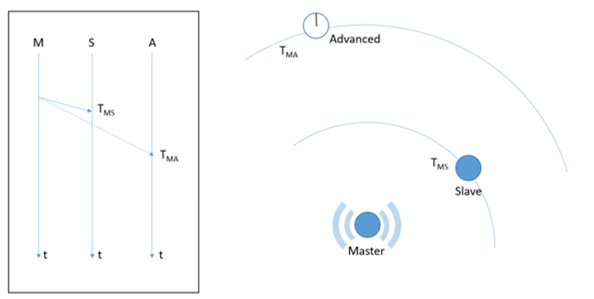
Figure 8: Ranging request, received by the Slave and the advanced mode radio at two different times.
As you can see in the diagram, the ranging request is sent by the Master and will arrive at the Slave at some time, TMS, and at the advanced mode radio at some other time, TMA. (Here, the subscripts indicate the radio role; TMA is, therefore, the time elapsed as the wave propagates from Master to the Advanced Ranging radio). In the inset image, we show the ranging request from the Master arriving at two different times: at the Slave and the advanced mode radios. (Note that the distance between the radios is not represented in the x-axis of this diagram – explaining the differing gradients of the propagation times).
Upon reception of the ranging request, the advanced mode radio will start its internal clock.
As with a conventional exchange, after an elapsed time of TMS (the time taken for the ranging request to arrive at the Slave) the Slave will synchronize with the incoming request and send back the ranging response. The ranging response then takes time, TMS again, to arrive back at the Master (assuming TMS = TSM). The ranging response from the Slave arrives at the advanced mode radio at some other time, TSA.
In the next diagram, the Slave sends the ranging response back to the Master after a delay of TMS (the time taken in the previous step) for the request to arrive at the Slave.
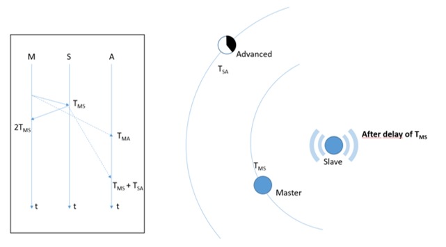
Figure 9: Ranging response sent from Salve to Master after a delay of TMS
When the ranging response arrives at the advanced mode radio, it stops its internal timer, recording the time difference between the arrival of the ranging request and the ranging response. The timing implications of this are shown below. Here we see the time difference, ΔT, measured by the advanced mode radio and how it relates to the Master-Slave, Slave-Advanced, and Master-Advanced delays.
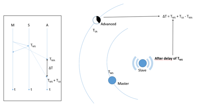
Figure 10: Expression for the Delay between Ranging Request and Ranging Response Measured by Advanced Ranging.
Looking more closely at this diagram, we can see that this gives us the geometric relationship between the various time differences and the ΔT timing measurement. This relationship is depicted below.
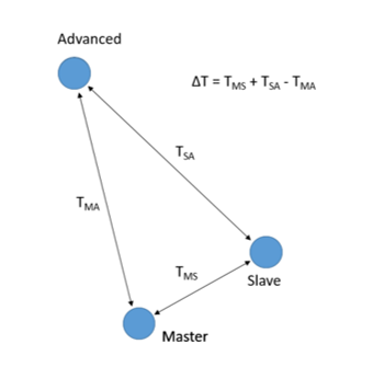
Figure 11: The geometric relationship between the times measured in Advanced Ranging.
Advanced Ranging for Localization
The extension of Advanced Ranging to localization is more complex than the conventional ranging case, and depends on which element of the system is attributed the Master, Slave, and Advanced Ranging roles. Below, we examine these three roles from the perspective of the tag.
Advanced Ranging Tag
In our first example, the Master and Slave are static anchors and the Advanced Ranging node is the tag to be located. We also add a third anchor, which does not take part in this first exchange.
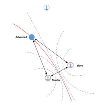
Figure 12: Advanced Ranging with the Advanced Ranging node to localize
The grey dotted lines represent lines of equal delay, ΔT, between the Master and Slave anchors. Thus, a single Advanced Ranging measurement places the Advanced-mode SX1280 on one of these curves of constant delay (which are hyperbolas, with the anchors at the foci).
To provide a location it is necessary, therefore, to perform additional time-difference measurements between additional anchors, as shown below, for the second time difference measurement—this time using a new combination of Master and Slave anchor nodes.
Note that, to obtain a 2D location, it is necessary to perform three time-difference measurements. Here is a representation of the second time-difference measurement for the same devices:
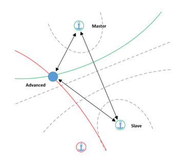
Figure 13: The Second Time-Difference Measurement in the Localisation Process
An important facet of this mode of operation is that an unlimited number of tags could theoretically listen to the Master-Slave exchanges between anchors—with important implications for the localization capacity of such a system. Where the tag object is to be located, this capacity is then only limited by the repatriation of the time difference measurements to the attendant network infrastructure. In the case of a tag locating itself, there is no such constraint.
Advanced Ranging Anchors
In this system, there is obvious scope for the anchors that are inactive to also assume the Advanced Ranging mode. However, it can be shown that overhearing information from the other anchors serves only to improve our knowledge of the location of the Master and Slave anchors.
Where the anchor locations are already known, additional information about their fixed locations is of no assistance in determining the location of the tag. Instead, it raises the possibility of our Advanced Ranging mode tag switching to Master or Slave mode, for a single ranging exchange, to improve our location knowledge.
GDOP Implications
Just as for RTToF ranging, the geometry of the anchor locations also determines localization accuracy. We plot the HDOP for the same scenario as before. Here we see that the area within that encircled by the anchors has a similar HDOP to the ranging case. The big difference is seen outside of this area. The HDOP outside is seen to rapidly increase, such that, over the same distance, where we saw a two-fold degradation in precision in Figure 7, we now see more than a twenty-fold degradation:
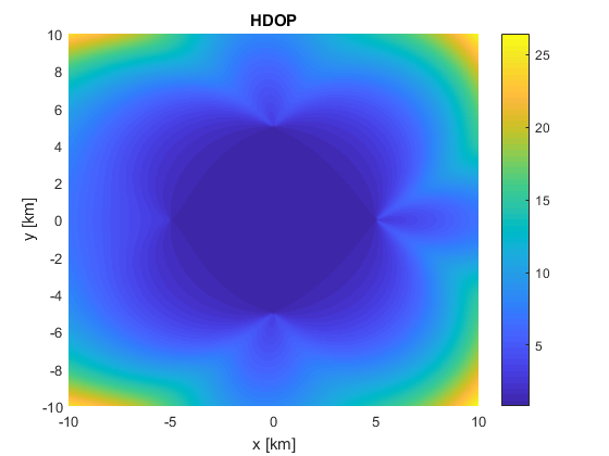
Figure 14: HDOP of Advanced Ranging
Summary
This mode of operation poses great gains in terms of capacity as the tag is a passive receiver of the ranging information. However, these gains come at the cost of a more complex localization problem with degraded HDOP at the periphery of the coverage area and, where applicable, the added management required for recovery of the time difference data from the tag.
Tag as Slave: Single Measurement
The alternative to operating the tag in advanced mode is to perform a conventional RTToF ranging exchange between the tag and a single anchor, with the remaining anchors within range in advanced mode. This situation is illustrated below:
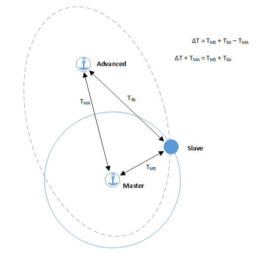
Figure 15: Advanced Ranging with the Tag in Slave Mode
As part of the fixed anchor infrastructure, the Master and advanced mode ranging node locations are known and concomitantly the Master-Advanced time, TMA, is also known. This means that the tag, instead of being located on a line of constant delay, is instead located on an ellipse with the two foci of which are the two anchor locations shown above by the grey dotted line.
We also have the RTToF measurement between Master and Slave, TMS, which further narrows the possible tag location to any intersection between the Advanced Ranging ellipse and RTToF circle (blue).
GDOP Implications
We examine again the HDOP of this scenario as shown in Figure 16. Here, we take our four-anchor localization system (based upon having the tag in Advanced Ranging mode). This time, however, we also include the influence of the single anchor (here the anchor on the right), which also performs the single Master-Slave distance measurement we outlined above.
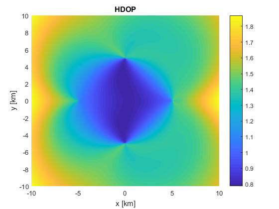
Figure 16: HDOP of Hybrid Ranging
A single ranging measurement reduces the HDOP back down to the same level we saw in the ranging-based solver—but with only a single (more costly) RTToF exchange. By virtue of the additional measurement, the single ranging measurement, aggregated with the Advanced Ranging measurements, results in a higher precision at the center of the HDOP plot than was possible in either previous example.
Summary
Here we see that we have much of the capacity advantage of the tag in Advanced Ranging mode—the ability of multiple nodes to receive the same exchanges increases the localization capacity of an Advanced Ranging based system. (Noting that spectral capacity may be required to uplink the ΔT measurement results, depending upon the architecture of the localization system). However, for the cost of an additional RTToF ranging exchange per-tag-localized, our HDOP improves by an order of magnitude. Our system HDOP becomes close to that described in the Ranging for Localization section above, where each ranging measurement required ranging exchanges between each tag and anchor.
Hybrid Modes of Operation
In this next example, to reduce the complexity of the solution, we show a hybrid technique combining tag-as-Slave and tag-as-Advanced Ranging techniques of the two previous examples to reduce the complexity of the solution back to solving for a single circle whilst using Advanced Ranging.
In the first step, anchor calibration, we perform what looks like one of the anchor-to-anchor exchanges we used our first Advanced Ranging localization steps. This gives us definite knowledge of channel and distance between our fixed anchors, TMS. (TSA and TMA can also be exploited for location.)
The subsequent phase, tag measurement, is a tag-as-Slave exchange from one Master anchor, the other listening in advanced mode. As we see from the figure above – we already know TMA’ = TMS of the previous, calibration measurement step.
Assuming the channel is unchanged in the interim between our measurements, we then have a perfect knowledge of both terms TMA’ and TMS’ of our Advanced Ranging equation. With only one unknown, we can therefore compensate both terms—reducing the equation to a direct measurement of the radius from Advanced anchor to Slave, TSA’.
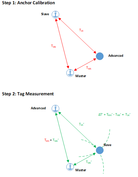
Figure 17: The two steps of a hybrid measurement where anchors and tag swap Slave and Advanced Ranging roles
Advanced Ranging for Proximity
Another interesting application of the SX1280’s Advanced Ranging functionality is to increase the accuracy of distance measurements by adding Advanced Ranging radios at the Master location. In a conventional ranging exchange, the Master initiates the ranging exchange with a slave and receives the synchronized response from the Slave, from which it can calculate the elapsed round-trip time of flight (a single result).
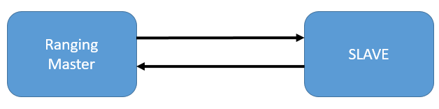
Figure 18: Conventional Master-Slave Round Trip Time of Flight Measurement, generating a single Result.
The basic principle of employing Advanced Ranging for enhanced proximity measurement is illustrated in the image below. We have already seen that, in Advanced Ranging mode, the radio can overhear the exchange between Master and Slave, timing the difference between the time of the Master’s request and the Slave’s response. In the case of an enhanced proximity measurement, we simply add Advanced Ranging radios in the same location as the Master.
The basic principle of employing Advanced Ranging for enhanced proximity measurement is illustrated in the image below. We have already seen that in Advanced Ranging mode the radio can overhear the exchange between Master and Slave, timing the difference between the time of the Master’s request and the Slave’s response. In the case of an enhanced proximity measurement, we simply add Advanced Ranging radios in the same location as the Master.
In the example below we have added three additional radios in Advanced Ranging mode. In this configuration, the Advanced Ranging radios are so close to the ranging Master that the Advanced Ranging radios' timers will start at a time equivalent to the Master’s start time. The principle here is that, where the Master-Slave RTToF Exchange is Overheard, Each Radio Generates a Ranging Result.
Similarly, the collocated Master and Advanced Ranging radios will all receive the ranging response from the Slave at the same time.
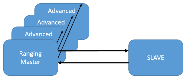
Figure 19. Using Advanced Ranging to Gather Multiple Ranging Results
The output of the four collocated radios is therefore four ranging distance measurements. However, with adequate antenna diversity, different multipath propagation paths may be taken, resulting in additional spatial diversity of the results. i.e., there are three additional and useful ranging results available for the cost of a single exchange from the perspective of the Slave’s energy consumption and the spectral occupation of the signal.